Geospatial | GeoHash | R-Tree | QuadTree
· Geospatial Data
· Spatial search problems
∘ K nearest neighbours
∘ Range and radius queries
· How spatial trees work
· Spatial Indexes
· R-tree
· K-d tree
· QuadTree
· Range queries in trees
· K nearest neighbours (kNN) queries
· Spatial Partitioning
· Spatial Partitioning + Indexing
· H3
· What’s GeoHash
∘ So does all the Geo-Hash library represent the flattened earth as 4 grids initially?
∘ So how can we use Geo-Hash in our use case?
∘ How Geohash works.
∘ Why does the Geo-Hash concept work?
· Use Cases for Geohashing
· Data partition strategies
· Uber Marketplace: Location Serving & Storage in the Uber Marketplace
∘ Driver/Rider location updates to the system
∘ Sharding Strategies
∘ City Sharding
∘ Geosharding
∘ Product Sharding
∘ Sharding Distribution
∘ Solution to Hotspots
∘ Location Storage
∘ Advance Topics [Todo]
· TODO
· References
Follow this link for all System design articles
Geospatial Data
- geospatial describes data that represents features or objects on the Earth’s surface.
- Records in a dataset have locational information tied to them such as coordinates, address, city, or postal code
Spatial search problems
- Spatial data has two fundamental query types: nearest neighbours and range queries. Both serve as a building block for many geometric and GIS problems.
K nearest neighbours
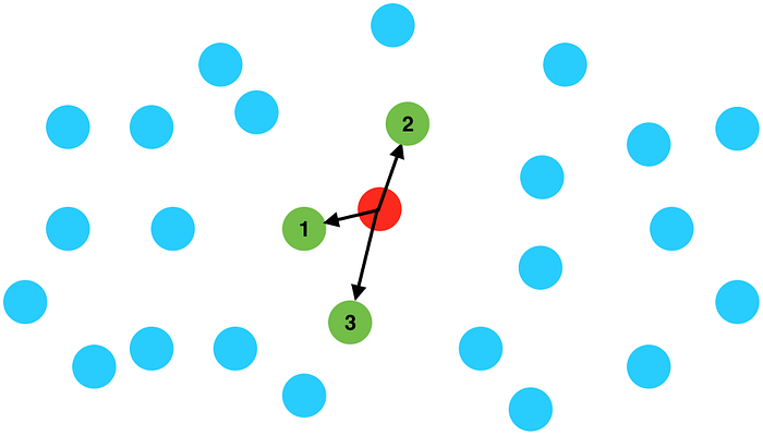
Given thousands of points, such as city locations, how do we retrieve the closest points to a given query point?
An intuitive way to do this is:
- Calculate the distances from the query point to every other point.
- Sort those points by distance.
- Return the first K items.
This is fine if we have a few hundred points. But if we have millions, these queries will be too slow to use in practice.
Range and radius queries

How do we retrieve all points inside…
- a rectangle? (range query)
- a circle? (radius query)
The naive approach is to loop through all the points. But this will fail if the database is big and gets thousands of queries per second.
How spatial trees work
Solving both problems at scale requires putting the points into a spatial index. Data changes are usually much less frequent than queries, so incurring an initial cost of processing data into an index is a fair price to pay for instant searches afterwards.
Almost all spatial data structures share the same principle to enable efficient search: branch and bound. It means arranging data in a tree-like structure that allows discarding branches at once if they do not fit our search criteria.
Spatial Indexes
Spatial indices are a family of algorithms that arrange geometric data for efficient search.
For example, doing queries like “return all buildings in this area”, “find 1000 closest gas stations to this point”, and returning results within milliseconds even when searching millions of objects.
- also immensely useful in many other tasks where performance is critical. In particular, processing telemetry data — e.g. matching millions of GPS speed samples against a road network to generate live traffic data for our navigation service.
- On the client-side, examples include placing labels on a map in real-time, and looking up map objects on a mouse
- R-Tree, QuadTree, Geohash, kd-tree,
- Fast lookup

- Substantial improvement in local performance, area 1% — 16%

R-tree
To see how this works, let’s start with a bunch of input points and sort them into 9 rectangular boxes with about the same number of points in each:

Now let’s take each box and sort it into 9 smaller boxes:

We’ll repeat the same process a few more times until the final boxes contain 9 points at most:


And now we’ve got an R-tree! This is arguably the most common spatial data structure. It’s used by all modern spatial databases and many game engines. R-tree is also implemented in my rbush JS library.
Besides points, R-tree can contain rectangles, which can, in turn, represent any kind of geometric object. It can also extend to 3 or more dimensions. But for simplicity, we’ll talk about 2D points in the rest of the article.
K-d tree
- K-d tree is another popular spatial data structure.
- kdbush JS library for static 2D point indices is based on it.
- K-d tree is similar to R-tree, but instead of sorting the points into several boxes at each tree level, we sort them into two halves (around a median point) — either left and right, or top and bottom, alternating between x and y split on each level. Like this:

Compared to R-tree, K-d tree can usually only contain points (not rectangles), and doesn’t handle adding and removing points. But it’s much easier to implement, and it’s very fast.
Both R-tree and K-d tree share the principle of partitioning data into axis-aligned tree nodes. So the search algorithms discussed below are the same for both trees.
QuadTree
A tree in which each node has four children can serve our purpose. Each node will represent a grid and will contain information about all the places in that grid. If a node reaches our limit of 500 places, we will break it down to create four child nodes under it and distribute places among them. In this way, all the leaf nodes will represent the grids that cannot be further broken down. So leaf nodes will keep a list of places with them. This tree structure in which each node can have four children is called a QuadTree

How will we build a QuadTree? We will start with one node that will represent the whole world in one grid. Since it will have more than 500 locations, we will break it down into four nodes and distribute locations among them. We will keep repeating this process with each child node until there are no nodes left with more than 500 locations.
How will we find the grid for a given location? We will start with the root node and search downward to find our required node/grid. At each step, we will see if the current node we are visiting has children. If it has, we will move to the child node that contains our desired location and repeat this process. If the node does not have any children, then that is our desired node.
How will we find neighbouring grids of a given grid? Since only leaf nodes contain a list of locations, we can connect all leaf nodes with a doubly-linked list. This way we can iterate forward or backwards among the neighbouring leaf nodes to find out our desired locations. Another approach for finding adjacent grids would be through parent nodes. We can keep a pointer in each node to access its parent, and since each parent node has pointers to all of its children, we can easily find siblings of a node. We can keep expanding our search for neighbouring grids by going up through the parent pointers.
Once we have nearby LocationIDs, we can query the backend database to find details about those places.
What will be the search workflow? We will first find the node that contains the user’s location. If that node has enough desired places, we can return them to the user. If not, we will keep expanding to the neighbouring nodes (either through the parent pointers or doubly linked list) until either we find the required number of places or exhaust our search based on the maximum radius.
How much memory will be needed to store the QuadTree? For each Place, if we cache only LocationID and Lat/Long, we would need 12GB to store all places.
24(8 bytes for LocationID, 8 bytes for Lat and 8 bytes for Long)
* 500M(assumption: unique locations)
=> 12 GB
Since each grid can have a maximum of 500 places, and we have 500M locations, how many total grids we will have?
500M / 500 => 1M gridsThis means we will have 1M leaf nodes and they will be holding 12GB of location data.
A QuadTree with 1M leaf nodes will have approximately 1/3rd internal nodes, and each internal node will have 4 pointers (for its children). If each pointer is 8 bytes, then the memory we need to store all internal nodes would be:
1M * 1/3 * 4 * 8 = 10 MBSo, the total memory required to hold the whole QuadTree would be 12.01GB. This can easily fit into a modern-day server.
How would we insert a new Place into our system? Whenever a new Place is added by a user, we need to insert it into the databases as well as in the QuadTree. If our tree resides on one server, it is easy to add a new Place, but if the QuadTree is distributed among different servers, first we need to find the grid/server of the new Place and then add it there (Check below Data partition strategies).
Replication and Fault Tolerance#
- Having replicas of QuadTree servers can provide an alternative to data partitioning.
- To distribute read traffic, we can have replicas of each QuadTree server.
- We can have a primary-secondary configuration where replicas (secondaries) will only serve read traffic; all write traffic will first go to the primary and then be applied to secondaries.
- Secondaries might not have some recently inserted places (a few milliseconds delay will be there), but this could be acceptable.
- What will happen when a QuadTree server dies? We can have a secondary replica of each server and, if the primary dies, it can take control after the failover. Both primary and secondary servers will have the same QuadTree structure.
What if both primary and secondary servers die at the same time?
- We have to allocate a new server and rebuild the same QuadTree on it.
- How can we do that, since we don’t know what places were kept on this server?
- The brute-force solution would be to iterate through the whole database and filter LocationIDs using our hash function to figure out all the required places that will be stored on this server.
- This would be inefficient and slow; also, during the time when the server is being rebuilt, we will not be able to serve any query from it, thus missing some places that should have been seen by users.
How can we efficiently retrieve a mapping between Places and the QuadTree server?
- We have to build a reverse index that will map all the Places to their QuadTree server.
- We can have a separate QuadTree Index server that will hold this information.
- We will need to build a HashMap where the ‘key’ is the QuadTree server number and the ‘value’ is a HashSet containing all the Places being kept on that QuadTree server.
- We need to store LocationID and Lat/Long with each place because information servers can build their QuadTrees through this.
- Notice that we are keeping Places’ data in a HashSet, this will enable us to add/remove Places from our index quickly.
- So now, whenever a QuadTree server needs to rebuild itself, it can simply ask the QuadTree Index server for all the Places it needs to store.
- This approach will surely be quite fast. We should also have a replica of the QuadTree Index server for fault tolerance. If a QuadTree Index server dies, it can always rebuild its index by iterating through the database.

Cache#
- To deal with hot Places, we can introduce a cache in front of our database.
- We can use an off-the-shelf solution like Memcache, which can store all data about hot places.
- Application servers, before hitting the backend database, can quickly check if the cache has that Place.
- Based on clients’ usage patterns, we can adjust how many cache servers we need.
- For cache eviction policy, Least Recently Used (LRU) seems suitable for our system.
Ranking#
How can we return to the most popular places within a given radius?
- Let’s assume we keep track of the overall popularity of each place.
- An aggregated number can represent this popularity in our system, e.g., how many stars a place gets out of ten (this would be an average of different rankings given by users)?
- We will store this number in the database as well as in the QuadTree. While searching for the top 100 places within a given radius, we can ask each partition of the QuadTree to return the top 100 places with maximum popularity.
- Then the aggregator server can determine the top 100 places among all the places returned by different partitions.
Remember that we didn’t build our system to update a place’s data frequently.
With this design, how can we modify the popularity of a place in our QuadTree?
- Although we can search a place and update its popularity in the QuadTree, it would take a lot of resources and can affect search requests and system throughput.
- Assuming the popularity of a place is not expected to reflect in the system within a few hours, we can decide to update it once or twice a day, especially when the load on the system is minimum.
Range queries in trees
A typical spatial tree looks like this:

Each node has a fixed number of children (in our R-tree example, 9). How deep is the resulting tree? For one million points, the tree height will equal ceil(log(1000000) / log(9)) = 7.
When performing a range search on such a tree, we can start from the top tree level and drill down, ignoring all the boxes that don’t intersect our query box. For a small query box, this means discarding all but a few boxes at each level of the tree. So getting the results won’t need much more than sixty box comparisons (7 * 9 = 63) instead of a million. Making it ~16000 times faster than a naive loop search in this case.
In academic terms, a range search in an R-tree takes O(K log(N)) time in average (where K is the number of results), compared to O(N) of a linear search. In other words, it’s extremely fast.
We chose 9 as the node size because it’s a good default, but as a rule of thumb, a higher value means faster indexing and slower queries, and vice versa.
K nearest neighbours (kNN) queries
Neighbors search is slightly harder. For a particular query point, how do we know which tree nodes to search for the closest points? We could make a radius query, but we don’t know which radius to pick — the closest point could be pretty far away. And doing many radius queries with an increasing radius in hopes of getting some results is inefficient.
To search a spatial tree for nearest neighbors, we’ll take advantage of another neat data structure — a priority queue. It allows keeping an ordered list of items with a very fast way to pull out the “smallest” one. I like to write things from scratch to understand how they work, so here’s the best ever priority queue JS library: tinyqueue.
Let’s take a look at our example R-tree again:

An intuitive observation: when we search a particular set of boxes for K closest points, the boxes that are closer to the query point are more likely to have the points we look for. To use that to our advantage, we start our search at the top level by arranging the biggest boxes into a queue in the order from nearest to farthest:

level 1 tree nodes
Next, we “open” the nearest box, removing it from the queue and putting all its children (smaller boxes) back into the queue alongside the bigger ones:

level 1 and 2 tree nodes mixed together
We go on like that, opening the nearest box each time and putting its children back into the queue. When the nearest item removed from the queue is an actual point, it’s guaranteed to be the nearest point. The second point from the top of the queue will be second nearest, and so on.

nodes of all levels (including points) mixed together
This comes from the fact that all boxes we didn’t yet open only contain points that are farther than the distance to this box, so any points we pull from the queue will be nearer than points in any remaining boxes:
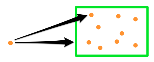
distance from a point to a box is a lower bound of distances to points within the box
If our spatial tree is well balanced (meaning the branches are approximately the same size), we’ll only have to deal with a handful of boxes — leaving all the rest unopened during the search. This makes this algorithm extremely fast.
For rbush, it’s implemented in rbush-knn module. For geographic points, I recently released another kNN library — geokdbush, which gracefully handles curvature of the Earth and date line wrapping. It deserves a separate article — it was the first time I ever applied calculus at work.
Spatial Partitioning
- Partitioning — essential to distributed processing Strategy: by spatial proximity
- Step 1: random sample
Step 2: build a tree
Step 3: leaf nodes → global partitioning - Strategies — Uniform grids, Quad-Tree, KDB-Tree, R-Tree, Voronoi diagram, Hilbert Curve

Spatial Partitioning + Indexing
- Distributed spatial indexing
- Global index — same tree in partitioning — bounding boxes
- Local index


H3
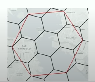
- Geospatial indexing system, a multi-precision hexagonal tiling of the sphere indexed with hierarchical linear indexes
- Created at uber, opened-source



What’s GeoHash
A geohash is a convenient way of expressing a location (anywhere in the world) using a short alphanumeric string, with greater precision obtained with longer strings.
Geo-Hash, it’s an encoding mechanism for a given location ( lat, long pair ).
Geohash is a geocoding system invented by Gustavo Niemeyer that allows us to know what area on a map a user is within. The user could be anywhere in that area, they are not necessarily in the center of the area.
- This is really useful as latitude and longitude only represent a single point on a map whereas a geohash describes a fixed area.3
- We can change the size of the area by specifying the number of characters in the hash from 1 to 10. Below from left to right, we can see the geohash area for 1,2 and 3 character hashes.

- Geohashing can also be used to provide a degree of anonymity as we don't need to expose the exact location of the user, depending on the length of the geohash we just know they are somewhere within an area.
- The core concept is to imagine the earth as a flattened surface & keep on dividing the surface into multiple grids (squares or rectangles, depending on implementation).

- In the following figure, we first divide the flattened earth surface into 4 grids represented by
0,1,2&3.
➡ Each grid now represents 4 different regions of a large size something like100_000 KM x 100_000 KM( this figure is just for understanding purposes, may not be accurate ).
➡ This is just too big to search for matching locations. So we need to divide it further — now we will divide each of those 4 grids into 4 parts — so the grid0now has 4 grids inside —00, 01, 02, 03; the figure shows grid 2 is divided into 4 parts —20, 21, 22, 23.
➡ Now say these smaller grids each represent an area of size20_000 KM x 20_000 KM.
➡This is still too big. So we keep on dividing each of these squares into further 4 parts & the process recursively continues till we reach a point where each region/grid can be represented as something like50 KM x 50 KMan area or some area which is suitable for our optimal searching.

So does all the Geo-Hash library represent the flattened earth as 4 grids initially?
➡ This is not necessary.
➡ Many of the Geo-Hash libraries takes a base of 32 alphanumeric characters & keeps on dividing the surface into 32 rectangles. You can implement your own Geo-Hash library with any base per see.
➡ But the core concept remains the same.
➡ In real life, we may need to compare existing Geo-hash libraries & see how good they are in terms of performance, APIs exposed & community support. ➡ In case they don’t fit our use case, we may need to write our own but chances are less. One good Geo-Hash library is Mapzen, take a look.
➡ Also remember that, in real life, cell/region dimensions may vary depending on longitude & latitude.
➡ It’s not all same area square or rectangles everywhere, nevertheless, the functionality remains the same.
So how can we use Geo-Hash in our use case?
➡We need to first decide on a length of Geo-Hash which gives us a suitable area something like 30 to 50 square KM to search for.

➡ Typically, depending on the Geo-Hash implementation, that length maybe 4 to 6 — basically, choose a length which can represent a reasonable search area & won’t result in hot shards.
➡ Let’s say we decide on the length L. We will use this L length prefix as our shard key & distribute the current object locations to those shards for better load distribution.
Constructing a geohash
The beauty of a geohash is in how it’s constructed. In brief, geo hashes are a type of grid spatial index, where the world is recursively divided into smaller and smaller grids with each additional bit.

Start with the entire planet, and divide it in half along the Prime Meridian — the first half containing latitudes in the range of (-180,0) as 0 and the second half containing the range (0,180) as 1. The half containing your point becomes the first bit.

Now, divide that half again along the Equator, and add the second bit. Repeat this subdivision, alternating between longitude and latitude, until the remaining area is within the precision desired. Finally, encode the resulting binary sequence using the geohash base 32 character map to create the final geohash string. For example, the longitude, latitude coordinate (37.77564, -122.41365) results in the binary sequence “0100110110010001111011110” and produces the geohash “9q8yy”.

Decoding a geohash
Another way of thinking about geo hashes are as interleaved longitude (even bits) and latitude (odd bits). This provides a simple method for converting a geohash back into longitude and latitude.

As above, each additional bit divides the area in half in a binary search. Latitude begins with a range of (-90, 90) degrees; the first bit of 1 reduces this to (0, 90); the second bit of 0 to (0, 45); the third bit of 1 to (22.5, 45); and so on until with the 12th bit, the range is (37.753, 37.797) with a midpoint of 37.775.
In this case, the width of the area encoded by 12 bits of latitude is +/- 0.022 degrees or approximately 2.4 km across at the equator. A longer geohash would encode more bits of precision; for example, increasing the geohash from 5 characters to 8 characters would increase latitude to 20 bits, reducing error to +/- 0.00085 degrees, or +/- 0.019 km.
Finding neighbours
As each character encodes additional precision, shared prefixes denote geographic proximity.

You might notice that all the California locations all begin with “9q”, and that Oakland and Berkeley share the “9q9p” prefix. Shared prefixes allow nearby locations to be identified through very simple string comparisons and efficient searching of indexes.
However, it is important to note the converse is not true! The London and Greenwich geo hashes are only about 6 km apart as the crow flies — but have no common prefix. This is because the Prime Meridian separates the two locations, dividing these two geo hashes with the very first flipped bit. Fortunately, it is straightforward to calculate the 8 neighbours for a given geohash. For example, the Southeast neighbour of “gcpv” is “u10h”, successfully jumping across this pesky imaginary boundary.
Searching an area
This method of expanding a geohash to include its neighbours can also be used to efficiently find the set of geohash prefixes to search an area. To find all prefixes within approximately 1 mile of the San Francisco geohash “9q8yykv551w”, first shorten the geohash to 6 characters, “9q8yyk”, then add in all 8 neighbors: 9q8yy7, 9q8yyt, 9q8yy5, 9q8yys, 9q8yym, 9q8yyj, 9q8yyk, 9q8yyh, 9q8yye. Any point in this area is known to start with one of these prefixes.

At Transitland, we use this property to specify simple bouding boxes for transit operators as part of a Onestop ID. For example, the SFMTA has over 3500 bus stops. As described above, it is quite possible that there is no common geohash prefix shared by every stop in the system (or, if there is, the be so short as to be limited usefulness). In the case of the SFMTA, only “9q” prefix is shared in common, which covers a very large portion of the Southwestern United States. However, the geohash prefix “9q8y”, when expanded to include neighbors, provides the 9 prefixes that can be used to find any stop, while covering a much smaller land area. This “neighbors implied” geohash is then used in the Onestop ID for SFMTA: “f-9q8y-sfmta”.
How Geohash works.
Geohash is a way of referring to any point on the earth with a single string of characters. It was invented in 2008 by Gustavo Niemeyer and GM Morton.
Geohash first splits the equator into 8 sections, each 45° of longitude wide. Then it splits the latitude into 4 sections, again each section 45° of latitude wide. This splits the world’s surface into these 32 regions.
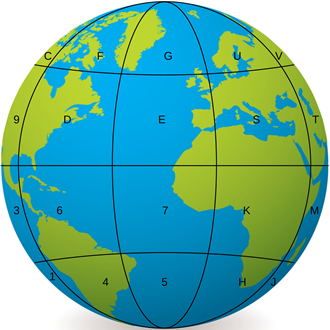
These 32 regions are labelled, using the 10 digits 0–9 and 22 letters (omitting A, I, L and O).
It is easier to see what is going on if we draw these regions on the sort of flat map we are used to.

The single character Geohash reference 6 identifies much of Latin America. Australia spans codes Q and R and China is mostly code W.
For more precision, we subdivide each of these large regions into smaller regions. Here we go down to level 2.
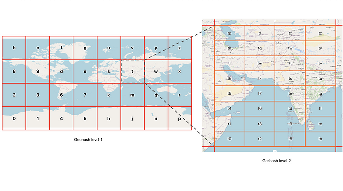
At level 3 you can see that Mysuru is in square tdn.

Precision
With 9 characters, the location can be specified as just under 5 m, which is sufficient for most purposes. But with up to 13 characters, you can specify a location within less than 5 mm.
How subdivisions are carried out
Level 1 splits a rectangular map of the earth into 32 rectangles 8 rectangles wide and 4 high. The splitting from Level 1 to Level 2 subdivides with new rectangles though this split is 4 rectangles wide and 8 high.
Subdividing from Level 2 to Level 3, the rectangles revert to 8 wide and 4 high. This alternating splitting is maintained throughout the levels. The result is that passing through 2 subdivisions a given area is split into 32 x 32 (ie 1024) subdivisions.
Z-shaped region labelling
Geohash regions are labelled in a Z-shaped order as shown.

This gives the best fit in terms of closeness between the Geohash, (a one-dimensional structure) and the surface of the world (which is two-dimensional).
Why does the Geo-Hash concept work?
- Geohashes use Base-32 alphabet encoding (characters can be 0 to 9 and A to Z, excl “A”, “I”, “L” and “O”)
- Imagine the world is divided into a grid with 32 cells. The first character in a geohash identifies the initial location as one of the 32 cells. This cell will also contain 32 cells, and each one of these will contain 32 cells (and so on repeatedly). Adding characters to the geohash sub-divides a cell, effectively zooming in to a more detailed area.
- As we saw Geo-Hash of a certain length represents an area of some finite square Kilometres.
- In the real world, only a finite number of cars or delivery agents or finite objects will fit in that area.
- So we can develop some estimations to figure out how many objects can be there in the worst case & calculate our index machine size accordingly which can reduce the hot shard possibility.
- Since we have a finite area with a finite number of objects, we won’t have a very hot shard anyway logically.
Use Cases for Geohashing
Geohashing was originally developed as a URL-shortening service but it is now commonly used for spatial indexing (or spatial binning), location searching, mashups and creating unique place identifiers.
A geohash is shorter than a regular address, or latitude and longitude coordinates, and therefore easier to share, remember and store.
- Social Networking — Used by dating apps to find romantic matches within a particular cell, and to create chat apps.
- Proximity Searches — Find nearby locations, and identify places of interest, restaurants, shops and accommodation establishments in an area.
- Digital Travels — Geohashers go on global expeditions to meet people and explore new places. The twist: the destination is a computer-generated geohash and participants in this turnkey travel experience have to write up and post their stories on the internet.
- Custom Interactive Apps — Geohashing can be used to create real-time, interactive apps.
Data partition strategies
With 20% growth(this is as per the problem statement) each year we will reach the memory limit of the server in the future. Also, what if one server cannot serve the desired read traffic? To resolve these issues, we must partition our QuadTree!(this can be any data structure but the Idea is how to handle partitions)
a. Sharding based on regions: We can divide our places into regions (like zip codes), such that all places belonging to a region will be stored on a fixed node. To store a place we will find the server through its region and, similarly, while querying for nearby places we will ask the region server that contains the user’s location. This approach has a couple of issues:
- What if a region becomes hot? There would be a lot of queries on the server holding that region, making it perform slow. This will affect the performance of our service.
- Over time, some regions can end up storing a lot of places compared to others. Hence, maintaining a uniform distribution of places, while regions are growing is quite difficult.
To recover from these situations, either we have to repartition our data or use consistent hashing.
b. Sharding based on LocationID: Our hash function will map each LocationID to a server where we will store that place. While building our QuadTree, we will iterate through all the places and calculate the hash of each LocationID to find a server where it would be stored. To find places near a location, we have to query all servers and each server will return a set of nearby places. A centralized server will aggregate these results to return them to the user.
Will we have different QuadTree structures on different partitions? Yes, this can happen since it is not guaranteed that we will have an equal number of places in any given grid on all partitions. However, we do make sure that all servers have approximately an equal number of Places. This different tree structure on different servers will not cause any issue though, as we will be searching all the neighbouring grids within the given radius on all partitions.
Uber Marketplace: Location Serving & Storage in the Uber Marketplace
Driver/Rider location updates to the system


Sharding Strategies
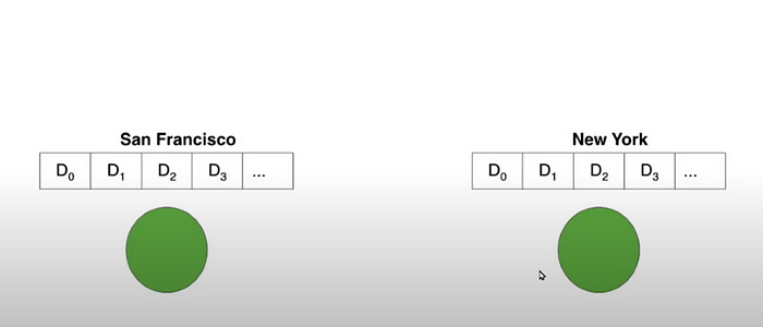
City Sharding
- Nodes are shared to have a particular city data
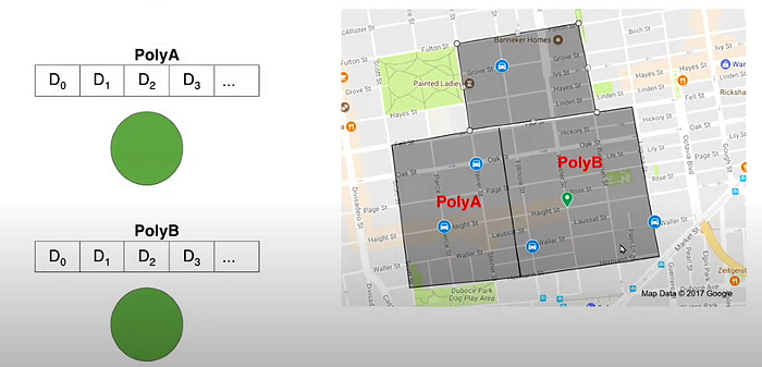
Geosharding
- take a map of the city and split it into different pieces.
- PolyA — hosted on node A
polyB — hosted on another node B
Product Sharding
- Split by city + product (xl, pool, mini)

Sharding Distribution


Solution to Hotspots
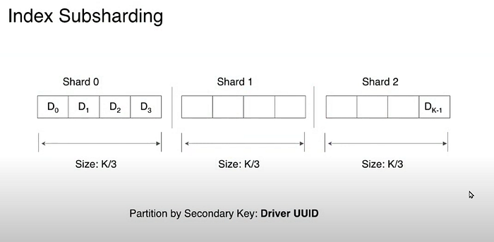

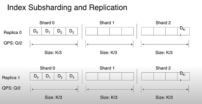


Location Storage


Advance Topics [Todo]
- Map Matching

2. H3
3. RingPop — Distributed Coordination

TODO
Buy me a coffee☕— https://ko-fi.com/tj007